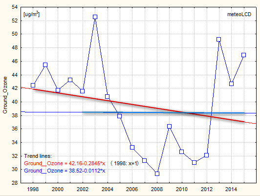
("bad ozone")
Mean and stdev of the year 2015: 46.9 +/- 34.4
Mean
+/- stdev:
1998 to 2015:
39.0 +/- 6.8 ug/m3
2002 to 2015: 36.0 +/- 6.1
Trends 1998 - 2015: -2.8 per decade
2002 -
2015: 0.1 per decade (flat trend line)
Watch the left scale to note that trends are very small!
("good ozone")
Mean and stdev of the year 2015: 324.2 +/- 42.7
minimum : 220.6 (5 Nov)
maximum: 445.6 (18 Apr)
Trendlines (start year is x =
1):
1998 to 2014: 312.08 +1.24*x (+12.4
DU/decade)
2002 to 2014:
332.04 - 0.26*x (- 2.6 DU/decade )
(Uccle
gives +0.95DU*y-1 for the 1998-2010 period)
(see also [16])
Calibration
multiplier to apply if Uccle Brewer #178 is the reference:
2015
: * 1.033 (provisional, many Uccle data not yet
available)
2015 common 107 days measurements
results:
Diekirch = 326.2 DU
Uccle DS = 337.6 DU (update when all Uccle data are available)
See [4] [8]
([8] shows strong
positive trend starting 1990 for
latitudes 45°-75° North, Europe): [27] give +1.32
DU/y at the Jungfraujoch for 1995-2004.
See also recent EGU2009 poster [16].

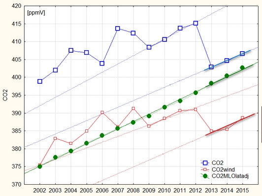
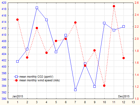
Mean and stdev of the year 2015: 407.6 +/- 4.9
The 1998-2001 data are too unreliable to be retained
for the trend analysis.
Trendlines (1998 is x = 1):
2002 to 2015: 403.0 + 0.40*x (+ 4.0 ppmV/decade)
2002 to 2012: 394.9 + 1.35*x (+ 13.5 ppmV/decade)
2013 to 2015:
372.9 + 1.87*x (+ 18.7 ppmV/decade)
The sharp plunge in 2013 should be taken with caution;
there also was a change in the calibration gas the 21 Jan. 2014
The Mauna Loa 2015 average is 400.83 ppmV, the trend for the 2013 to 2015
period is about 15 ppmV/decade [34]
The German Hohenpeissenberg trend for the 2010 to 2015 period is 17 ppmV/decade,
very close to the 2013-2015 meteoLCD trend of 18.7[48]
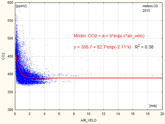
The second picture shows the asymptotic CO2 values
(CO2wind)
derived from the model published in [21] .
The blue upper curve shows the yearly mean
values at Diekirch; the middle red curve the
asymptotic CO2 values that would exist if wind velocity was infinite, and
the lower green curve the yearly averages at
Mauna Loa, augmented by +1.8 ppmV to respect the latitudinal gradient of
approx. 0.06 ppm per degree.
The yearly trends calculated from the yearly mean and the asymptotic values
at Diekirch are very similar to the MLO trend of 2.08 for the last 3 years:
MLO:
+2.08 ppmV/year
Diekirch CO2: +1.87 ppmV/year
Diekirch CO2wind: +1.90 ppmV/year
Trends are also similar for the period 2009 to 2012 (see the thin trend lines).
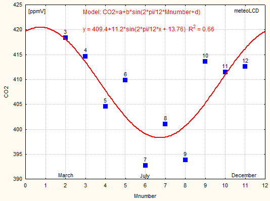
The CO2 data (monthly averages) clearly show the summer-time lows and
winter highs, which reflect the impact of variable seasonal photo-synthesis (see here). This simple 12
month periodic sinus pattern was also found in 2014.
Actually, as shown in addendum 3, the CO2 lowering intensity of wind
speed seems to be an important modifier of this pattern (as visible from the low CO2
values during the Jan and Feb months), possibly masking the effect (or
better: the non-effect) of photosynthesis.
If we omit the Jan and Feb months, we find the "classic" sine wave, with an amplitude of 11 ppmV (or a total swing of 22 ppmV), which is close to the 20 ppmV found at the stations Hohenpeissenberg (HPB) and Ochsenkopf (OXK) in 2013. The 12 month periodic sinus model is rather good, with an R2=0.66.
 .
.
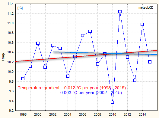
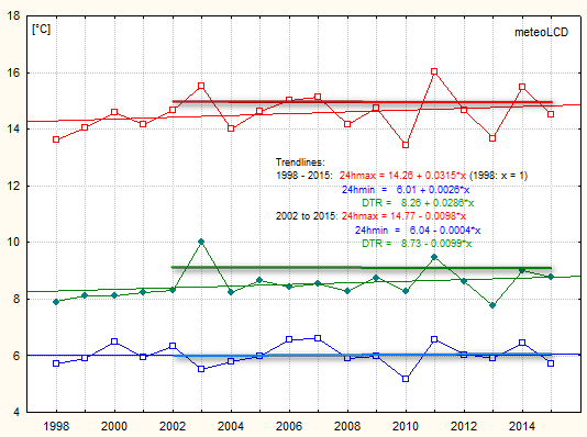
Mean and stdev of the year 2015
(from monthly averages):
Diekirch: 10.15 +/- 5.72 (10.20 from all half-hour readings)
Findel: 10.36 +/- 6.48
Mean temperatures (+/- stdev):
1998 to 2015 :
10.33 +/- 0.46 °C
2002 to 2015 :
10.37 +/- 0.49 °C
2006 to 2015 : 10.40 +/- 0.56 °C (last decade)
The
sensor location has not been moved since 2002! The old thermistor sensor has
been replaced by a PT100
(see comments in 2015_only.xls).
Trends from 2002 to 2015:
meteoLCD: -0.03°C/decade
Findel:
+0.11°C/decade
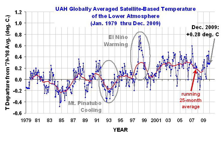
Latest Global temperature anomaly trends for same period:
UAH (satellite) : + 0.05°C/decade [45]
RSS (satellite) : - 0.062°C/decade
CRU (Hadcrut4): + 0.013°C/decade
Highest decadal Central England warming trend from 1691 to 2009:
+1.86°C/decade for 1694-1703!
See also [15] (which may be obsolete)
Range (DTR) [°C]
DTR = daily max - daily min temperature
Mean and stdev of the year 2015 (from monthly
averages):
Diekirch: 8.76 +/- 3.36 (8.79 from all half-hour readings)
Findel: 7.75 +/- 2.81
Mean DTR (
+/- stdev):
1998 to 2015: 8.53 +/-
0.55
2002 to 2015: 8.65 +/- 0.57
2006 to 2015: 8.59 +/- 0.47 (last decade)
For 2002 to 2015: all trends are practically flat.
Findel DTR trend is flat from 2004 to 2015.
A fingerprint of climate warming is that daily minima increase more
rapidly than
daily maxima so that the DTR trend should become negative. Clearly the
data do not show this neither at Diekirch nor at the Findel.
The BEST data set for Luxembourg [29] stops at
2013.
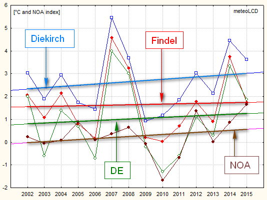
Values of DJF temperature of the year 2015:
Diekirch: 3.63
Findel: 1.73
Contrary to what is often suggested in the media, winters were cooling since 2002 to 2013. The cooling trend (about -0.5 °C/decade) has now reversed into a slight warming.
Diekirch: +0.5 °C/decade since
2002
Findel: +0.1 °C/decade
Germany: +0.3 °C/decade [46]
NOA: +0.5 °C/decade
(NOA normalized index)
The plot shows the mean temperatures of
December (from previous year), January and February. It also shows in
brown the NAO index for the months Dec to Feb [47]
The North Atlantic Oscillation clearly
influences our winters (but note the 2014 year exception!); the correlations between the 3 different DJF
temperature series
and NAO normalized index are 0.54, 0.40 and 0.60, all except the second (Findel) significant at the 5% level. The NAO
index trend is
equal to the Diekirch trend.
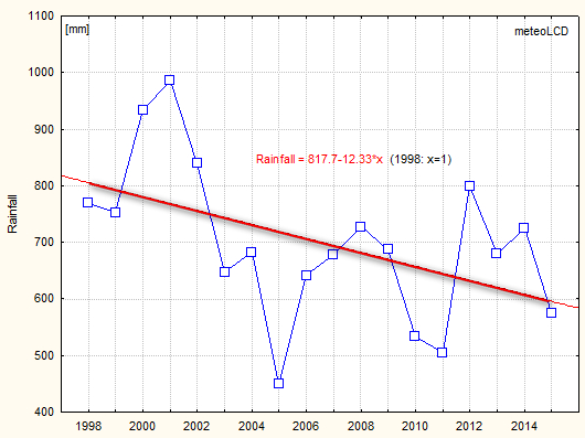
Values of rainfall (precipitation) of the year 2015:
Diekirch: 575.6
Findel: 630.4
1998 to 2015 mean +/- stdev: 700.7 +/- 138.4 mm
2002 to 2015 mean +/-stdev: 655.1 +/_108.9 mm
The negative trend from 1998 to 2015 seems spectacular:
-123.5 mm/decade, which comes from the very high values of 2000 and 2001.
The 2002-2015 period suggests a more constant pattern and shows a much lower trend
of -28.5 mm/decade.
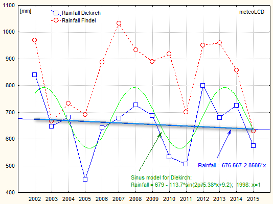
Clearly precipitation shows an oscillation pattern, so linear trends
should be taken with precaution.. A good model for the Diekirch data is
a sinus function of 5.38 years period (R2 = 0.54) (see lower
graph).
The same model suggests a similar period of 5.78
years for the Findel precipitation pattern (R2 = 0.43)
[6] gives short term periods of 6 to 7 years for
the Western European region.
Values of total solar energy
of the year 2015:
Diekirch: 1127.3 KWh/m2
Uccle: 1111.7 [49]
1998 to 2015 mean: 123.92 W/m2 = 1085.5 kWh/m2
2002 to 2015 mean: 124.02 W/m2 = 1086.4 kWh/m2
Visible negative trend:
1998 to 2015: -17.6 kWhm-2/decade
(not surprising with exceptional 2003 peak!)
Nearly flat trend from
2004 to 2015 : -1.8 kWhm-2/decade
(actual solar cycle #24 begins Jan. 2009).
(see
Addendum 1 for calculations of radiative
forcing and solar sensitivity, addendum 2 for
detecting a solar influence on temperature and moist enthalpy)
Helioclim satellite measurements show ongoing solar dimming over
Luxembourg for 1985 to 2005 [33] (see
graph)
[14] finds 0.7 Wm-2y-1
for West-Europe 1994-2003 , meteoLCD +1 Wm-2y-1 for
1998-2003.See also [9]

(meteoLCD values derived from pyranometer data by Olivieri's method)
Values of sunshine hours
of the year 2015:
Diekirch: 1550 hours (215m asl)
Findel: 1796 hours
(365m asl, Campbell- Stokes)
Trier:
1652 hours (279m asl)
[40]
(Diekirch total used for missing May data)
Uccle: 1734 hours (100m asl)
Negative trends:
1998 to 2015: - 116 hours/decade
2004 to 2015: - 35 hours/decade
Note that negative trend has diminished (nearly flat since 2004).
The decline from 2012 to 2013 is -10.8%, to be compared to the data from the Fraunhofer Institut which give a decline of -10.6 % of the German PV "Volllasttunden" [37]
See paper
[23] by F. Massen
comparing 4 different methods to compute sunshine duration from pyranometer
The next graph shows the plots of the four above-mentioned stations. It should be noted that meteoLCD (Diekirch) is located in a valley, Findel and Trier on top of a plateau. The Findel totals are much higher than those of the other stations, which certainly is also partially caused by the use of the Campbell-Stokes instrument known to give too high readings (in July and August the excess of Findel readings was highest). The 2006 and 2007 Uccle values should be taken with caution!
From 2007 on all 4 stations give totals that vary in the same manner (synchronous increase and decrease)


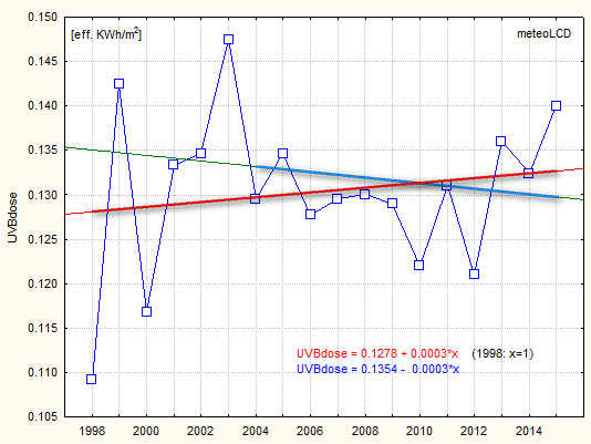
Erythemal UVB dose of the year 2015: 0.140 KWh/m2
mean +/- stdev:
1998 to 2015: 0.130 +/- 0.009 eff. kWh*m-2y-1
2002 to 2015: 0.132 +/- 0.009
All trends are
practically flat!
See
[10]
and [22] (poster finds slight
positive trend in June (+2%) and negative trend in August (-1%), no trend
for other months, for period 1991 to 2008)
(The slight negative trend in biologically effective UVB is not consistent with
the slight negative trend of the total ozone column [28],
[50] , but consistent with the small
decrease of solar irradiance since 2004).
UVA dose of the year 2015: 50.54 KWh/m2
mean +/- stdev:
1998 to 2015 53.8 +/- 4.6 kWh*m-2*y-1
2004 to 2015: 53.9 +/- 4.2
Overall trend is flat, from 2004 to 2015 slightly negative.
The 3 independent measures of solar energy, UVB and UVA doses all point to a slight solar dimming since 2004.

Mean moist enthalpy of 2015: 26.01+/- 11.32 kJ/kg
See [24] on how the energy content of moist air is
calculated. Several authors, (e.g. Prof. Roger Pielke Sr.) insist that air
temperature is a poor metric for global warming/cooling, and that the energy
content of the moist air and/or the Ocean Heat Content (OHC) are better
metrics
Mean yearly moist enthalpy values are very close, but they may change from
zero up to 60 KJ/kg during a year. Moist enthalpy can not be
calculated for temperatures <= 0 °C.
mean +/- stdev:
2002 to 2015
27.78 +/- 0.96 kJ/kg
2004 to 2015: 27.60 +/- 0.92
Both trends are clearly negative which is consistent with
the trends in temperature and solar energy. during the 14 years.
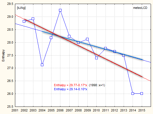
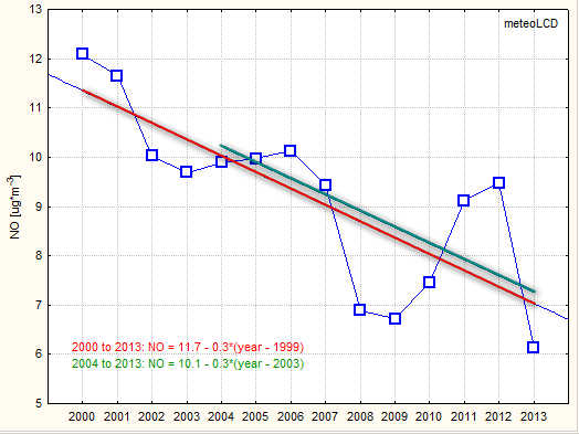
(end of measurements in 2014. This part will not be updated anymore!)
The 1998-1999 data are too unreliable to be retained.
2000 to 2013: trend: - 0.3 ug*m-3*y-1
2004 to 2013 rend: idem
mean +/- stdev:
2000 to 2013: 9.2 +/- 1.8 ug/m3
2004 to 2014: 8.5 +/- 1.5
Many missing data from 2011 to 2013 ( 25%, 21% , 8%) so be careful! All
these concentrations are very low! Luxembourg-City has a background of 25-30
and rural Vianden (Niklausberg) one of 2.5 (approx. 2013 values from
[39])
see [11] which gives ~30% reduction from 1990 to 2005 for the EU-15 countries.
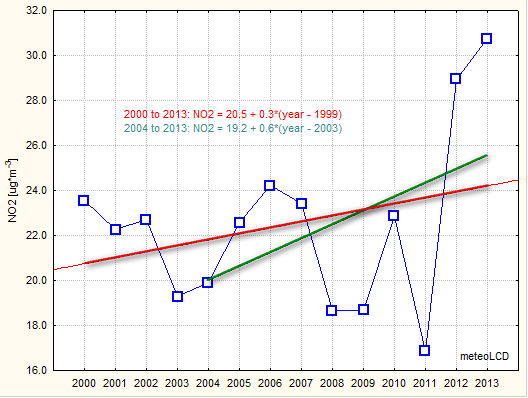
(end of measurements in 2014. This part will not be updated anymore!)
The 1998-1999 data are too unreliable to be retained.
2000 to 2013: trend: + 0.3 ug*m-3*y-1
2004 to 2013 rend: + 0.6
mean +/- stdev:
2000 to 2013: 22.5 +/- 3.9 ug/m3
2004 to 2014: 22.7 +/- 4.5
Many missing data from 2011 to 2013 ( 25%, 21% , 8%) so be careful! All these concentrations are low! Luxembourg-City has a background of 58 and rural Vianden (Niklausberg) one of 9.4 (average since 1988) [38]


