
The software UV_CALC has been used with its default parameters

The mean difference is -0.026 eff. W/m2, the standard deviation = 0.043 (1333 data points)

MODEL and MEASUREMENT
a comparison of computed and measured eff. UVB irradiation
Francis Massen (Physics Lab, LCD; meteoLCD) and Nico Harpes (Radioprotection Office)
file: uvcalc.html
version 1.01 02 July 2002
Abstract:
A comparison is made between effective UVB irradiance computed by the UV_CALC
software from YES and the UVB irradiance measured by a Solar Light broadband UVB
biometer. A good agreement can be found under blue sky conditions, when the
tropospheric and total ozone data as well as the cloud cover percentage are
taken into account; differences become great when sky is cloudy. Using the
software with its default parameters gives much poorer results.
Index:
| 1 | The UV_CALC software from Yankee Environmental Systems (YES) |
| 2 | Comparing the measurements with the calculations using default parameters |
| 3 | Comparing the measurements with the calculations using actual parameters |
| 4 | Using the UV_CALC with measured ozone for blue sky days ( i.e.0% cloud cover) only |
| 5 | Conclusion |
| References |
1. The UV_CALC.EXE
software from Yankee Environmental Systems (YES)
For many years YES
sells a software package called UV_CALC
[1] to compute the effective UVB irradiance and the daily effective UVB
dose; in this paper we use the MSDOS version 1.2 from 1991. This software is
based on Green's model [2] to compute the effective UVB irradiance on a
given day, at a given location (longitude, latitude, altitude) and under
specified atmospheric conditions: height ( and thicknesses) of tropospheric and
stratospheric ozone layers, AOT and cloud cover. Despite its age and
primitive user interface, the program is easy to use: a given run produces a
graphical output of the eff. UVB irradiance over the day, and generates an ASCII
file with the irradiances, the cumulutive dose and the various parameters used.
A serious lack is the restriction to a single day-only run; the user who wishes
to compute a whole month or extended period of time will have to repeat the
program execution for every day, or do some programming to achieve this.
Before doing its calculation, the software asks for several parameters:
- date and time
- location and altitude
- low level ozone layer: thickness ( in DU) and aerosol thickness ( in km)
- high level ozone layer: thickness (in DU), altitude and aerosol thickness of
that layer
- cloud cover ( on percent)
The default values for the low level ozone layer are 18 DU and 1.4 km AOT; they
are 304 DU, 22.4 km and 0.0045 km AOT for the higher layer parameters.
At meteoLCD (http://meteo.lcd.lu) both ground ozone concentration ( in ug/m3,
altitude 215m asl) and total ozone column are measured; the AOT is measured only
at the 1020 nm wavelength. A serious problem is that the software asks for a
ground layer ozone thickness in DU, which can not be readily derived from our
ground-based concentration measurements in ug/m3. We choose for this paper to
divide the ug/m3 concentration by 4 to get an approximative DUlow
thickness; this DUlow was substracted from our total ozone DU
(measured by a Microtops II spectrophotometer) to give the DUhigh.
All the other parameters (AOT's) were left unchanged, with the exception of the
cloud cover. We introduced 3 cases: 0% for blue sky, 75% for a "many
clouds" condition, and 95% for a "heavy clouds" condition. These
conditions appear in the table
of the DU data on the meteoLCD web-site.
2. Using the UV_CALC with all its default parameter values
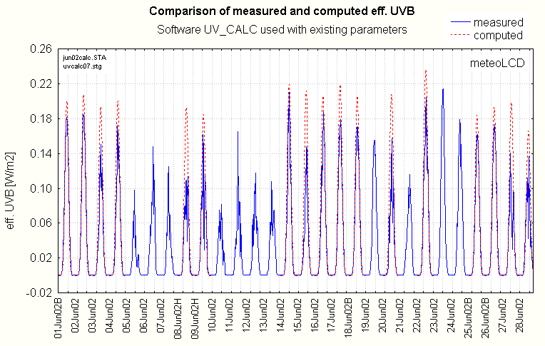
This comparion was made on data from the 01 to 28 June 2002 (1333 cases); the following graphs show the UVB irradiance during that period and the relation-ship between measured and computed data.
|
Variations of computed and
measured eff. UVB irradiance from 1st to 28 June 2002; the days ending in
B are blue sky days (0% cloud cover), those ending in H represent an
approx. 95% cloud cover situation. The software UV_CALC has been used with its default parameters |
|
As expected, the differences
between the measured and computed data are in general smallest under blue
sky conditions, and highest under 95% cloud cover. The mean difference is -0.026 eff. W/m2, the standard deviation = 0.043 (1333 data points) |
|
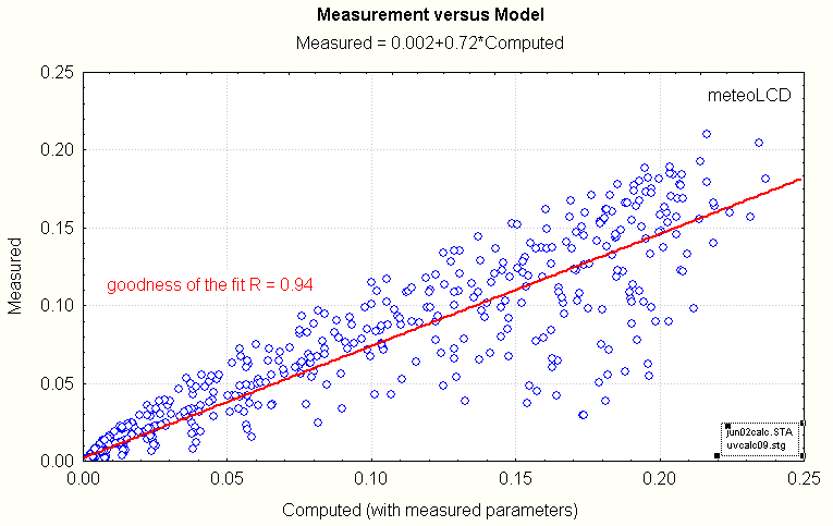
Plotting the measured data against the computed shows that the latter are always too high and that the deviations become very large at high UVB irradiances. The goodness of the fit is R = 0.896 |
3.
Using the UV_CALC with measured ozone and cloud cover parameter
As said above, meteoLCD measures ground ozone concentration in ug/m3 as well
as the thicknes of the total ozone column ( in DU). These parameters are entered
into UV_CALC (taking 0.25*ground-ozone in ug/m3 as the thickness in DU of that
lower layer), as well as the cloud cover ( 0%= blue sky, 15% = light haze,
75%=many clouds, 95%=heavy clouds).
The following graphs show this new comparisons:
 |
As the ozone data total ozone column) are not available for every day, we have only 805 computed data points- |
 |
As above, the difference is smallest under blue sky conditions; the mean difference is -0.013, and the standard deviation = 0.027, both values are much smaller than in the previous case where the default parameters have been used. So it pays off to use measured ozone data (even if the low layer thickness has been computed by dividing the ground ozone concentration by 4; only a vertical ozone profile could give the correct thickness of the lower layer) |
 |
The graph of the measured versus the computed data shows a much lesser spreading, and a much better slope of 0.72 (against 0.56; 1 would be the ideal case). The goodness of the fit is R = 0.94, much higher than in the preceeding case |
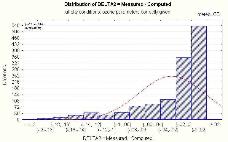 |
The statistical distribution of the differences between measured and computed data is highly left-skewed; the majority ( ~68%) of the differences are in the [-0.02; + 0.02] range. |
A conclusion from point 2 and 3 is that when using UV_CALC, one should use
whenever possible, real data for the various parameters. This gives a much
better result than simply applying the default "typical" parameters,
even if the conversion of gound ozone concentration in ug/m3 to thickness of
that layer use uin this paper is debatable.
4. Using the UV_CALC with measured ozone for blue sky days ( i.e.0% cloud cover) only
Finally, the comparison will be made on the 4 blue sky days ( i.e. days with a 0% cloud cover); as expected, this situation (0% cloud cover, actual ozone parameters in UV_CALC) gives the best results: mean difference = - 0.0004, standard deviation = 0.012. plotting the measured versus versus the computed data shows only small spreading; if UV_CALC is used with its default parameters, the mean difference = -0.014 and the standard deviation = 0.024. Using the true ozone situation thus betters the mean difference by a factor of 3.5
 |
The linear fit gives a slope of 0.891; this is the multiplier to apply to the computed data to yield a "correct" result under blue sky conditions. |
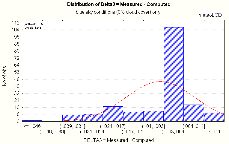 |
The distribution of the differences between measured and computed data is less skewed than in the previous case; about 56% of the differences lie in the quite narrow range [-0.003.. + 0.004] |
In summary:
| situation | uv_calc used with | mean +/- SD of the difference between measured and computed data | multiplier to apply to computed data and goodness of fit R |
| all data | default parameters | -0.026 +/- 0.043 | 0.56 0.90 |
| all data | actual ozone and cloud-cover | -0.013 +/- 0.027 | 0.72 0.94 |
| blue sky data only | default parameters | -0.014 +/- 0.024 | 0.75 0.99 |
| blue sky data only | actual ozone and cloud-cover | -0.0004 +/- 0.012 | 0.89 0.99 |
| 5.
Conclusion
The UV_CALC software is a valuable tool to asset the working of a UV
sensor measuring the eff. UVB irradiance, if the actual ozone
conditions and cloud cover are at least approximately given as input
parameters. If feasible, one should limit the comparisons to blue sky ( 0%
cloud cover) days. Computing a fit between measured and observed data
gives a good multiplier which can be applied to fill the gaps in the
measurement series in the case of a sensor breakdown; UV_CALC could also
be useful to calibrate (with all the needed caveats!) a sensor with
unknown specifications to correct eff. UVB [3]. |
| 1 | General Description of UV_CALC v. 1.2 |
| 2 | Green, Mo and Miller, Photochem. Photobiol. 20, 473 (1974) |
| 3 | Personal email correspondance (June 2002) with Dr. Nada Jallo from the Hashemite University of Jordan concerning the Delta-T UVB sensor |
| 4 | Prof. Dr. Gunther Seckmeyer, Institute of Meteorology and Climatology, University of Hannover: personal communication 29June2002 |