COVID-19 LUXEMBOURG
by Francis Massen (francis.massen@education.lu)
06 June 2020
1. Introduction
The COVID-19 pandemic (or epidemic) started the 29th Feb 2020 in Luxembourg; this is day 0 or day 1, dependent on counting (I start at day 0).
I wanted to follow the evolution using a model (better: a formula) developed about 200 years ago by Benjamin GOMPERTZ, an English autodidact and later member of the Royal Society. The GOMPERTZ formula belongs to the category of sigmoid functions, which describe a phenomenon starting slowly, going through a quasi exponential development phase and than slowing down up to zero progression. The formula written in Excel notation is:
y = a*exp(-b*exp(-c*x)) with exp(x) = ex
It has only 3 parameters, and clearly a represents an horizontal asymptote when x tends to infinity: y(inf) = a*exp(-b*0) = a
The Gompertz function is much in use in population dynamics, but also in the first phase of a developing epidemic.
All data and graphs are in the subdirectory Archive.
2. The situation at the end (31-May-20)
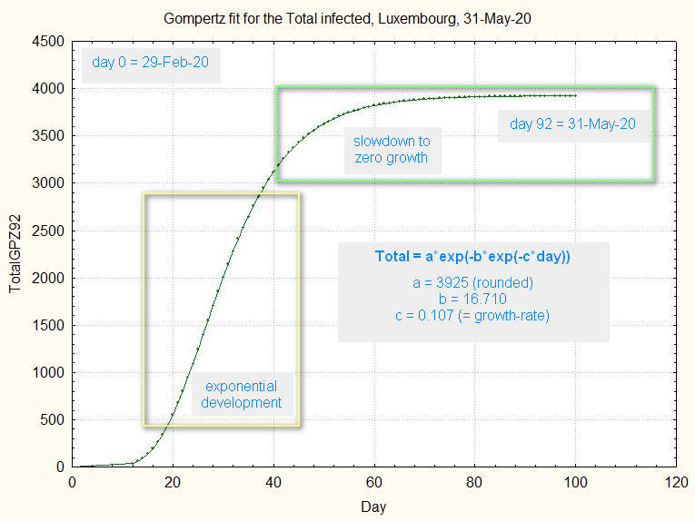
Fig.1 shows the Gompertz function modelled on the 92 days of the total infected in Luxembourg, starting 29-Feb-20 and ending 31-May-20.
Modeling means that the parameters a, b and c are mathematically choosen by a regression calculus (Levenberg-Marquardt algorithm) to give a best fit to the observations:
fig.1. Gompertz function fitted to the total infected after 92 days, extended to 100 days.
The next figure shows the previous fit and the observations:
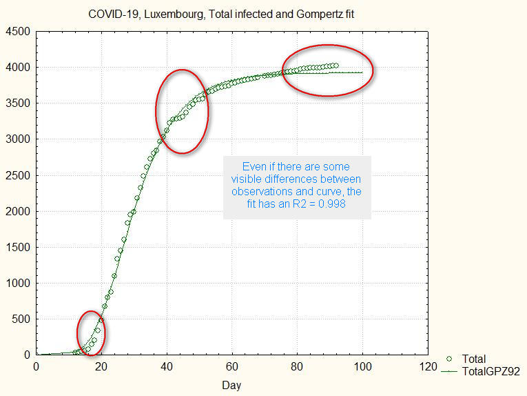
fig.2. Deviations from Gompertz fit
Despite the visible differences, statistically all parameters are significant and the goodness of the fit R2 = 0.998 (the maximum possible is R2=1).
3. How does the Gompertz function fit at the start?
A first question is "when is the fit statistically significant?".
Let's take as an example the situation on 16-Mar. None of the 3 parameters were statistically significant; the uncertainty range for parameter a was a ridicule [-19621 ... +22437 ]
Nevertheless the fit to the few data points was visually excellent:
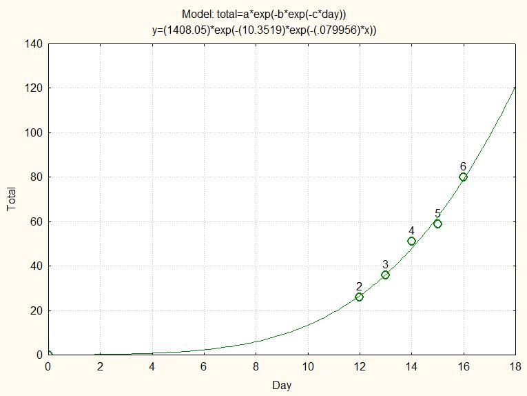
fig.3 Gompertz fit to the 6 available data from 29-Feb to 16-Mar
If we would have taken this fit as a valid predictor for the future, we would have been in for a big surprise:
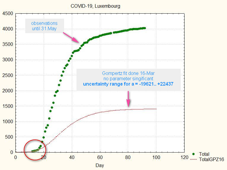
fig.4. The previous fit extended to 100 days (red line), compared to the observations (green dots).
The green curve shows what happened, the red is the predictor made the 16-May.
Conclusion #1: beware of predictions made too early in the development of the epidemic!
The 24-March (=day 24) was the first day where all parameters were statistically significant (alpha = 95%); if we use the Gompertz function calculated from the available data at that moment, the previous fig.4 will change (see fig.5):
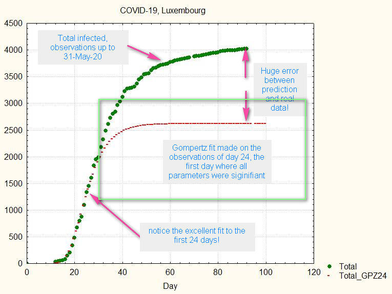
fig.5. Gompertz fit made at day 24; the uncertainty range for a at that date shown by the green box was [1182 .. 3098]
We see that the number of total infected is finally 1400 more that the prediction made the 24th March; the final total is even about 1000 cases more than the higher bound of the uncertainty range!
Conclusion #2: beware of predictions made too early in the development of the epidemic! (I repeat myself!)
4. Evolution of the number of death
Fig.6 shows the number of deaths on the first day where all parameters of the Gompertz fut are significant; the yellow rectangle corresponds to the borders of the uncertainty range, which is large, but not impossible large.
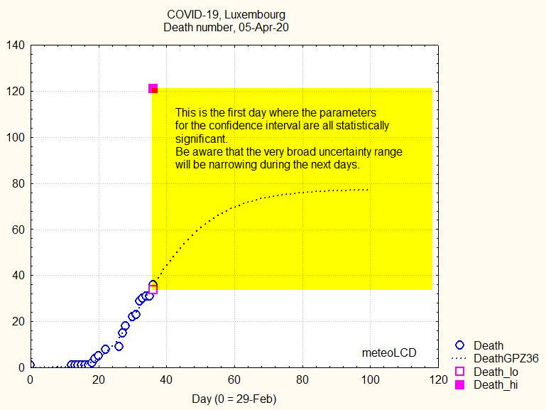
Fig.6. Death number of Gompertz curve prediction, 05-Apr-20 (=36th day)
The Gompertz curve does not fit very well, as the death number increases by jumps:
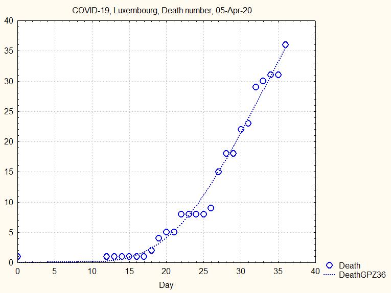
Fig.7. Death number and Gompertz fit on all observations until 5th Apr. 20
The uncertainty range does not narrow smoothly, but goes through some violent swings before narrowing continously from about the 44th day ( 8 April) on, as shown by the next animation:
Fig. 8. Animation showing the evolution of death number and the uncertainty interval (upper and lower bounds by full and open squares)
Similar to what has been concluded above: if one had taken the prediction made the 9th April, the number of predicted deaths would have been about 250, to be compared to the final 110.
Conclusion #3: beware of predictions made too early in the development of the epidemic! (I repeat myself!)
5. Final remarks
1. The 200 year-old Gompertz curve represents well the ongoing epidemic, independent from the political decisions to impose strict measures like shutting down schools and many economic actors, and imposing a relatively strict quarantine: the evolution of both total infected and total death number follows well this simple curve. The death numbers vary more by pause and jumps, so that deviation from the Gompertz curve is more apparent.
2. Even if all 3 parameters of the curve are found to be statistically significant, one can not rely on the prediction to have a correct estimate of the total number of infections and of death. These predictions are only valid when enough data are present, which represents a serious decision problem as this "enough" number is unknown a priori. In hindcast, one can see that after about 50 days the total number of infected can be reasonable well predicted; this is the moment where the exponential increase is over and the progression begins to slow down. For the number of deaths the date where a valid prediction can be made is about 10 days later (i.e. 60 days after the start).
3. The sad conclusion is that this modeling, independent from its intellectual and scientific interest, is a poor instrument to help making political decisions at the earliest moment, a time when they are most urgently needed. Models are very good at the final development stages of the pandemic; but alas their usefulness is inversely proportional to the delay from the start of the epidemic. One should not be fooled by an extremely good R2: all models follow the past in an excellent way, but this is in general no guaranty on how good they are in predicting the future.
Francis Massen, meteoLCD
06 June 2020