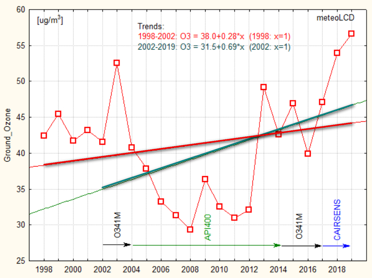
("bad ozone")
Mean +/-stdev
of
2019: 56.6 +/- 38.4 ug/m3
Mean
+/- stdev (from yearly means)
1998 to 2019:
41.3 +/- 7.8 ug/m3
2002 to 2019: 40.8 +/- 8.6
Trends 1998 - 2018: 38.32+0.28*x (almost flat)
2002 -
2018: 34.98+0.69*x
(be
careful: API400 values may be too low!)
Please note the succession of 3 different instruments; after the
definitive breakdown of the Teledyne API400, the old O341M sensor from Environnement SA was used again
and finally replaced by a
CAIRSENS O3&NO2 in 2018. As NO2 values are below the minimum of this
instrument, readings can be taken as O3 only. A comparison has shown an
excellent concordance with the official Beckerich station.
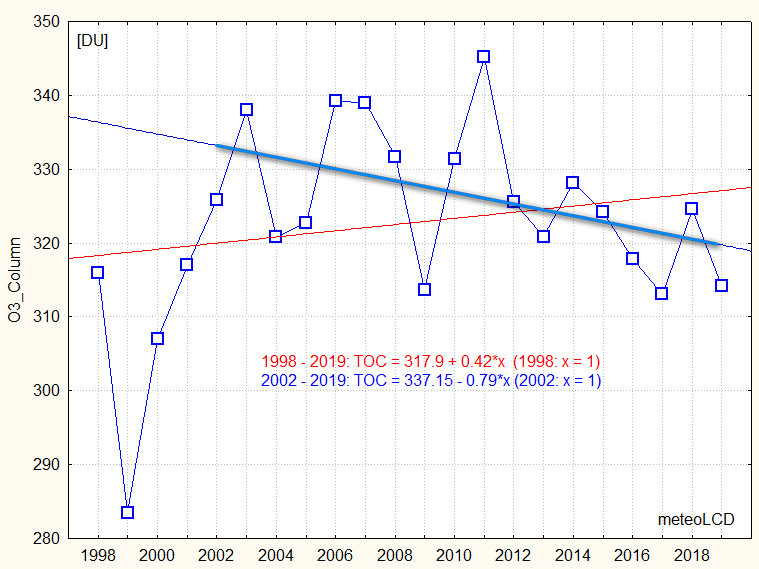
("good ozone")
Mean and stdev of the year 2019: 313.0 +/- 39.0 DU
minimum : 222.3 (16 Fep)
maximum: 451.3 (11 Mar)
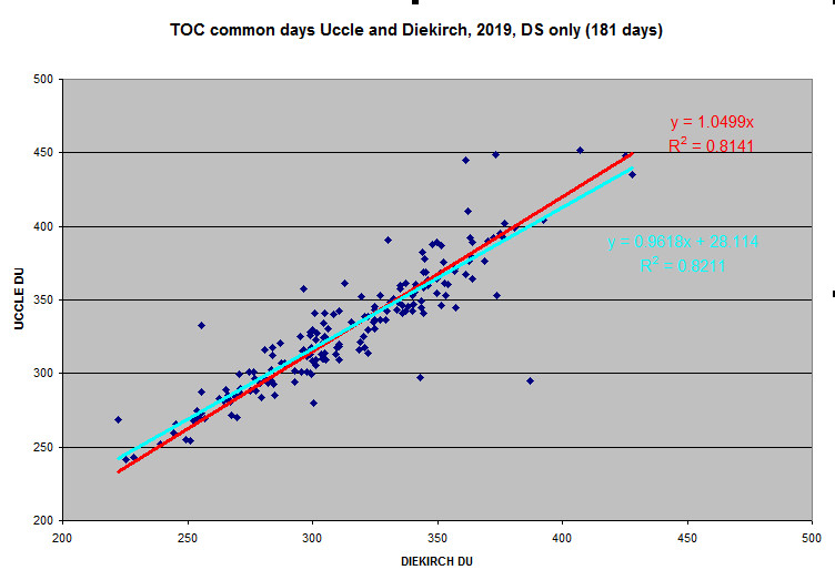
181 common day
direct sun readings for 2019 at Uccle and Diekirch:
Diekirch
: 314.20 +/- 38.95
Uccle (Brewer 178): 330.38 +/- 41.24
After 3 years of slight thinning, the TOC is
again increasing.
Trendlines (start year is x =
1):
1998 to 2019:
(+4
DU/decade)
2002 to 2019:
(- 8 DU/decade )
Uccle
has
a slight positive trend of +3.6 DU/decade for the 1998-2019 period, and a
similar of +3.9 DU/decade from 2010 to 2019.(see also
[16])
Calibration
multiplier to apply to the Diekirch DU data
[55] and
[56]
if Uccle Brewer 178 is the reference: 1.0499 (R2 =0.81)
See [4] [8]
([8] shows strong
positive trend starting 1990 for
latitudes 45°-75° North, Europe): [27] give +1.32
DU/y at the Jungfraujoch for 1995-2004.
See also recent EGU2009 poster [16].
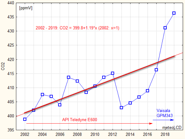
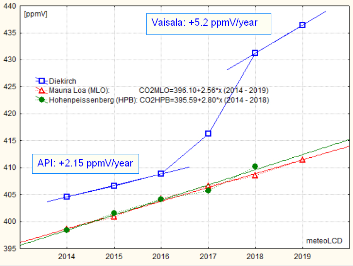
Attention: The instrument for measuring CO2 (API Teledine E600) has been replaced by a Vaisala GMP343 sensor the 27 Jun 2017. The jump from 2017 to 2018 seems implausible high, so a zero bias should be considered possible!
Mean and stdev of the year 2019: 434.4 +/- 31.7 ppmV
The 1998-2001 data are too unreliable to be retained
for the trend analysis.
Trends :
2002 to 2019: 1.19 ppmV*y-1
The sharp plunge in 2013 should be taken with caution;
there also was a change in the calibration gas the 21 Jan. 2014.
The second picture zooms on the last 6 years, and
gives the readings of Diekirch (DIK), Mauna Loa (MLO) and Hohenpeissenberg (HPB)
from 2014 to 2019; 2019 data are not yet available for HPB. Note the very
different elevations! Mauna Loa has no vegetation at all, Diekirch and HPB
similar grass and forests.
The yearly trends are for this period are
| Diekirch 219m asl semi-rural |
+ 2.15 (API) +5.2 (Vaisala) ppmV/year |
|
| Hohenpeissenberg (HPB) 977m asl, forests |
+ 2.80 ppmV/year | [48] [57] |
| Manua Loa (MLO) 3397m asl, no vegetation |
+ 2.56 ppmV/year | [34] [57] |
Be careful with the Vaisala readings, as the Vaisala GPM343 might not give the same accuracy as the former API! These readings also are given for local atm. pressure and un-dried air!
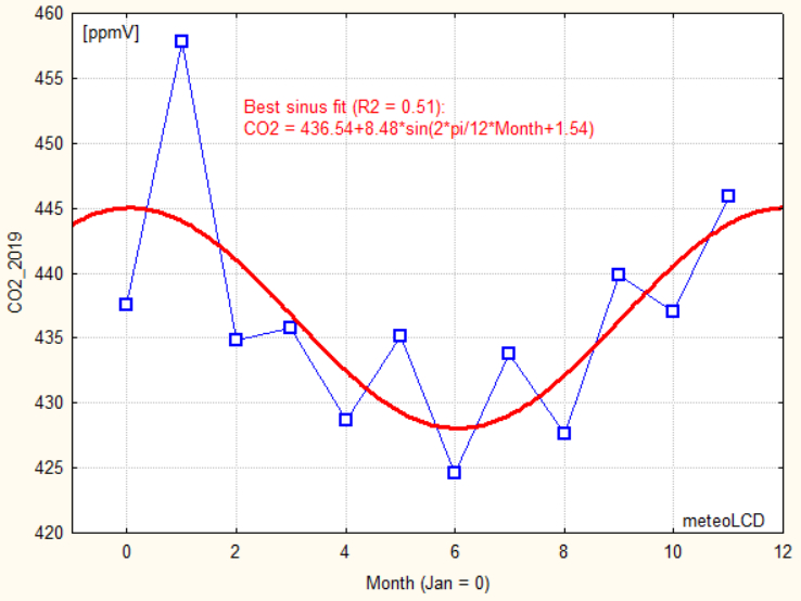
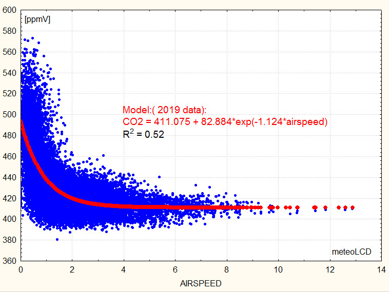
The CO2 data (monthly averages) show the summer-time lows, which reflect the impact of variable seasonal photo-synthesis (see here). A simple 12 month periodic sinus pattern was also found in 2014 and 2015. Actually, as shown in addendum 3, the CO2 lowering intensity of wind speed seems to be an important modifier of this pattern, possibly masking the effect (or better: the non-effect) of photosynthesis. This happened in 2016 and 2017. This year the yearly amplitude of the sinus fit is 8.48 ppmV (a total swing of ~17 ppmV, to be compared to about 15 ppmV at the HPB station [48]).
See the end of addendum 3 for a picture of CO2 versus windspeed.
 .
.
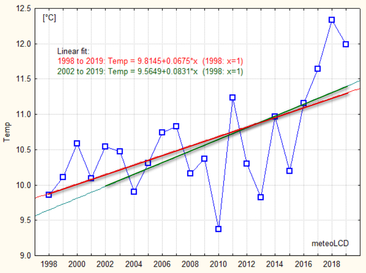
Mean and stdev of the year 2019
(from monthly averages):
Diekirch: 11.96 +/- 6.35
Findel: 10.68 +/- 6.59
Mean Diekirch temperatures (+/- stdev) from yearly averages:
1998 to 2019 :
10.59 +/- 0.73 °C
2002 to 2019 : 10.69 +/- 0.77 °C
2010 to 2019 : 10.90 +/- 0.96 °C (last decade)
The
sensor location has not been moved since 2002! Sensor is a PT100
(see comments in
2015_only.xls); new 4-20mA
amplifier (with calibration) installed the 4th May 2016.
Trends from 2002 to 2019 (be aware that 2018 was a very strong El Nino year!):
meteoLCD: +0.070 °C/year
Findel: +0.048
°C/year
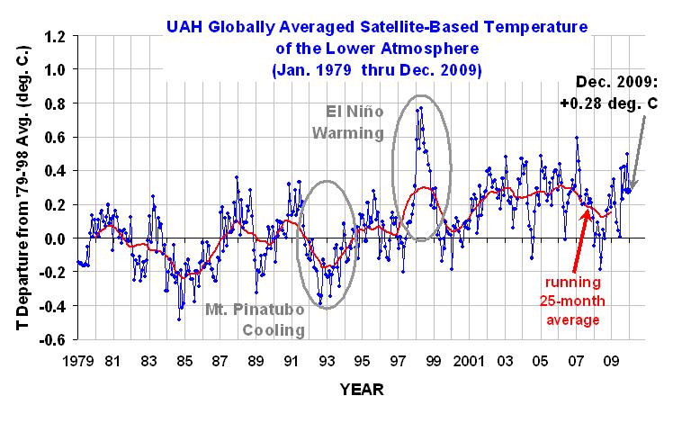
Latest Global temperature anomaly trends for same period 2002-2018:
UAH (satellite, LTT): + 0.0123°C/year
[45]
RSS (satellite, LTT) : + 0.0172°C/year
CRU (Hadcrut4krig v2): + 0.0164°C/year
Highest decadal Central England warming trend from 1691 to 2009:
+1.86°C/decade for 1694-1703!
See also
[15] (which may be obsolete)
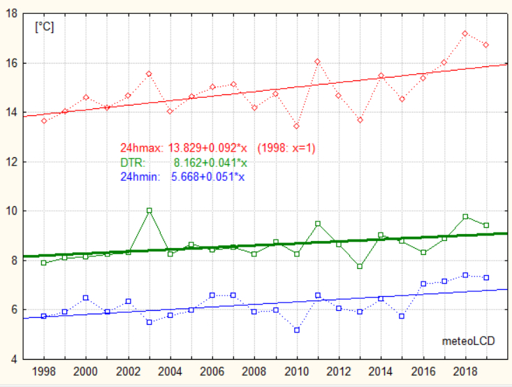
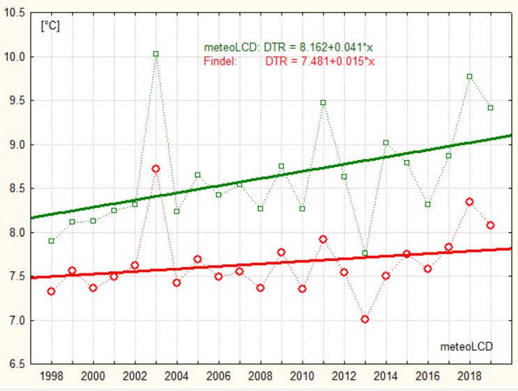
Range (DTR) [°C]
DTR = daily max - daily min temperature
Mean and stdev of the year 2019 (from monthly
averages):
Diekirch: 9.43 +/- 3.25
Findel: 8.08 +/- 2.55
Mean DTR at Diekirch:
1998 to 2019: 8.63
2002 to 2019: 8.75
2010 to 2019: 8.83 (last decade)
For 1998 to 2018: all trends are positive, the 24hmin
trend is lower than the 24hmax trend.
A fingerprint of climate warming is that daily minima increase more
rapidly than
daily maxima so that the DTR trend should become negative. This
fingerprint does not exist here (and neither at the Findel station, see 2nd plot).
The BEST observational data set for Luxembourg
[29] stops at
2013. For our latitude of 50° North, BEST shows a positive DTR trend for the
period 1988 to 2011, whereas theCMIP5 multi-model mean gives a similar but
negative trend... so much for the concordance between climate models and
observations! (graph
here).
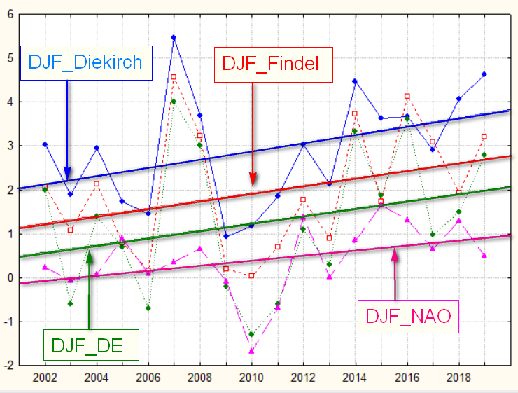
Values of winter DJF temperature of the year 2019:
Diekirch: 4.62
Findel: 1.93
NOA: 0.65 NAO normalized index [47]
The trends show warming winters since 2002 to 2018, with the warming probably caused by the NAO.
Trends from 2002 to 2018:
(2016 was a very strong El Nino year!):
Diekirch: +0.095 °C/year since
2002
Findel: +0.086
Germany: +0.084 [46]
NAO: +0.058
The plot shows the mean temperatures from
December (of previous year) to February. It also shows in
magenta the NAO index for the months Dec to Feb
The North Atlantic Oscillation clearly influences
our winters (but note the exception for the strong 2016 El Nino year!
[51]); the correlations between all the DJF
temperature series
and the NAO_DJF normalized index is statistically significant (=0.59) at the 5% level.
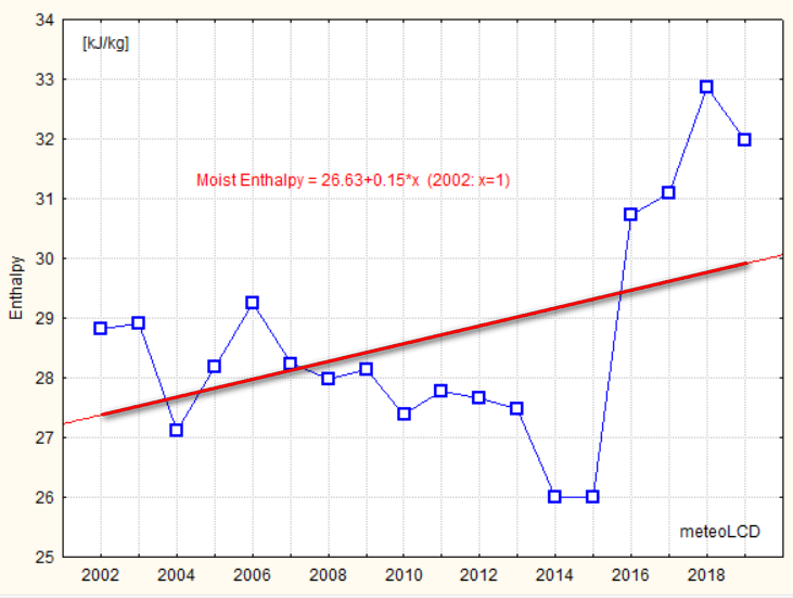
Mean moist enthalpy of 2019: 31.98 +/- 15.34 kJ/kg
See [24] on how the energy content of moist air is
calculated. Several authors, (e.g. Prof. Roger Pielke Sr.) insist that air
temperature is a poor metric for global warming/cooling, and that the energy
content of the moist air and/or the Ocean Heat Content (OHC) are better
metrics.
Mean yearly moist enthalpy values are mostly very close, but they may change from
zero up to 60 KJ/kg during a year. Moist enthalpy can not be
calculated for temperatures <= 0 °C.
mean +/- stdev from
2002 to 2019:
28.65 +/- 1.90 kJ/kg
Trend is slightly positive from 2002 to 2019; the 2016 "monster" El Nino extended into 2017 .
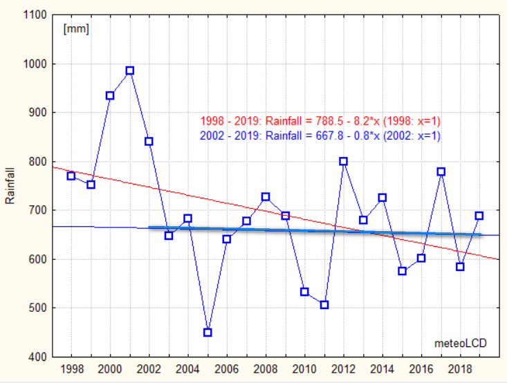
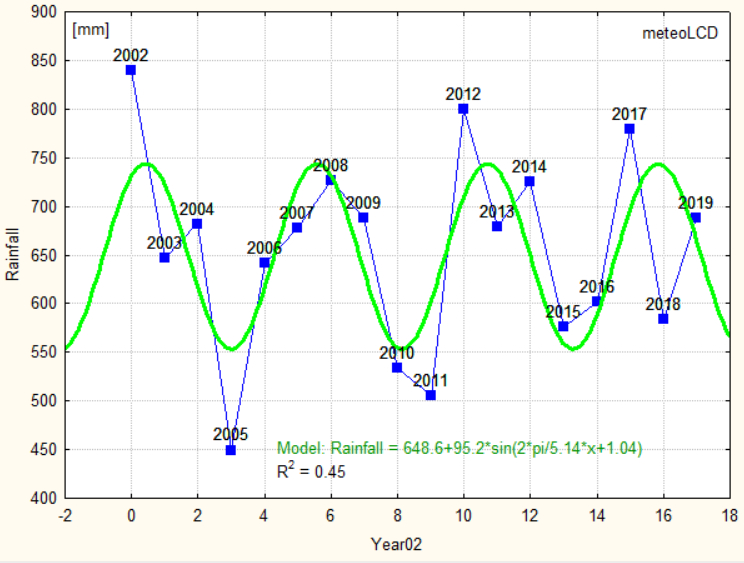
Values of rainfall (precipitation) of the year 2019:
Diekirch: 687.6 mm
Findel: 779.2 mm
1998 - 2019 mean +/- stdev: 693.9 +/- 129.9 mm
2002 - 2019 mean +/-stdev: 657.0 +/- 102.4 mm
The negative trend from 1998 to 2018 seems spectacular:
-82 mm/decade, caused by the very high values of 2000 and 2001.
The 2002-2019 period has a pratically zero trend!
Clearly precipitation shows an oscillation pattern, so linear trends should be taken with precaution (or simply seen as non-sensical).
A good model for the Diekirch data is a
sinus function: the calculation
(Levenberg-Marquart algorithm)
suggests for the interval 2002 - 2019 a 5.14 years period (~62 months, R2 =
0.45);
in the model x = 0 corresponds to 2002), with a mean value of 649 mm and an
amplitude of 95 mm; the phase shift of 1.04 rad is close to 1/6 period. All
these values are close to those of the preceding year.
[6] gives short term periods of 6 to 7 years for
the Western European region.
The oscillatory rainfall pattern is a good example how foolish it is to apply linear regressions to data when these are harmonic, something the media, activist groups and many politicians often do without much thinking.
Values of total solar energy
of the year 2019:
Diekirch: 1172.6 KWh/m2
1998 to 2019 mean +/- stdev: 1115.7 +/- 48.8 kWh/m2
2002 to 2019 mean +/- stdev: 1115.7 +/- 52.8 kWh/m2
Trends from 1998 to 2019 is nearly flat, and relative important (+9.11 kWh*m-2*y-1)
for last decade. [52]
(see
Addendum 1 for calculations of radiative
forcing and solar sensitivity, addendum 2 for
detecting a solar influence on temperature and moist enthalpy)
Helioclim satellite measurements show ongoing solar dimming over
Luxembourg for 1985 to 2005 [33] (see
graph)
[14] finds 0.7 Wm-2y-1
for West-Europe 1994-2003 , meteoLCD +1 Wm-2y-1 for
1998-2003.See also [9]
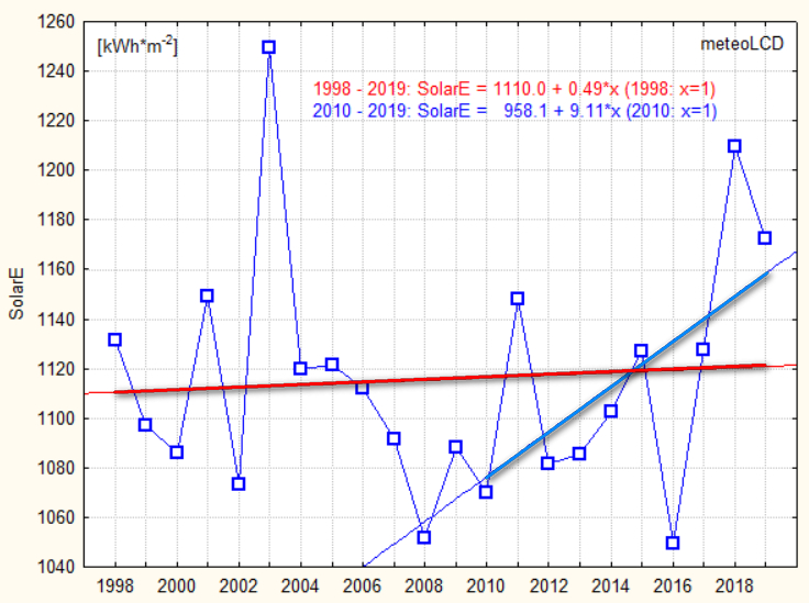
(meteoLCD values derived from pyranometer data by Olivieri's method)
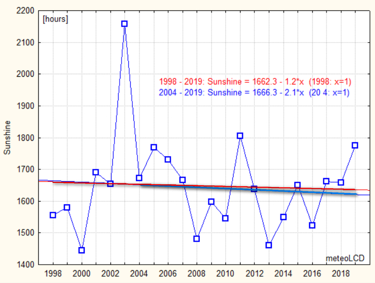
Values of sunshine hours
of the year 2019:
Diekirch: 1776 hours (215m asl)
(from pyranometer)
Findel: 1975 hours
(365m asl, (from Campbell- Stokes)
Trier: 1935 hours (279m asl)
[40]
[53]
(Petrisberg)
Maastricht: 1926 hours (114m asl)
[53]
Very small negative trends:
1998 to 2019: - 12 hours/decade
2004 to 2019: - 21 hours/decade
The decline from 2015 to 2017 is clearly visible in
the German PV electricity production, but the negative trend reverses for
the very sunny year 2018 [58].
See paper
[23] by F. Massen
comparing 4 different methods to compute sunshine duration from pyranometer
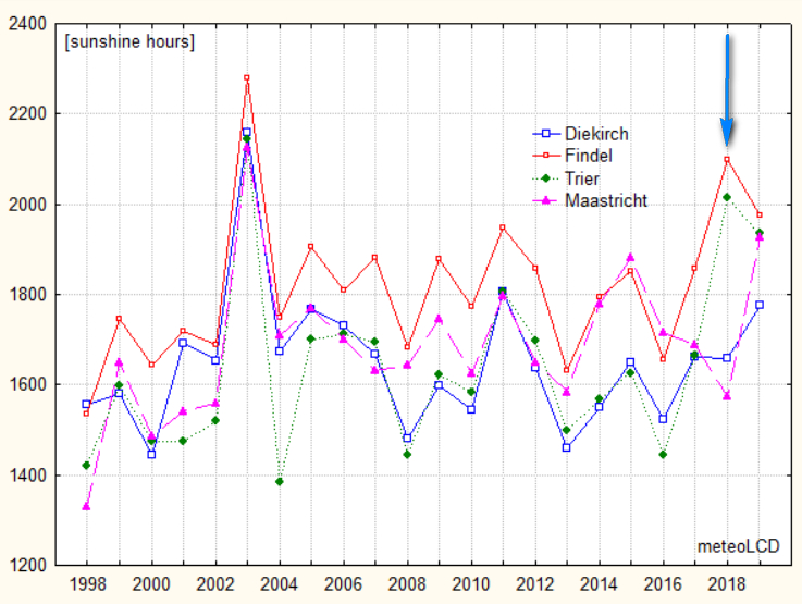
The 2nd graph shows the plots of the four above-mentioned stations. It should be noted that meteoLCD (Diekirch) is located in a valley, Findel, Trier and Maastricht airport on top of a plateau. The Findel totals are much higher than those of the other stations, which certainly is also partially caused by the use of the Campbell-Stokes instrument known to give too high readings (in July and August the excess of Findel readings was highest).
All 4 stations give totals that practically always vary in the same manner (synchronous increase and decrease). But notice how the readings in 2018 between the 2 groups (Diekirch, Maastricht) and (Findel, Trier) are quite different (blue arrow)!
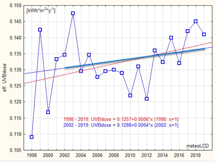
Erythemal UVB dose of the year 2019: 0.141 kWh/m2
mean +/- stdev:
1999 to 2019: 0.133 +/- 0.008 eff. kWh*m-2y-1
2002 to 2019: 0.134 +/- 0.007
2010 to 2019: 0.134 +/- 0.008 (last decade)
The trend over
2002 - 2019 is slightly positive, the trend line from 1998 to 2019 should be
taken with a grain of salt, as the 1998 readings seem abnormally low.
.
See
[10]
and [22] (poster finds slight
positive trend in June (+2%) and negative trend in August (-1%), no trend
for other months, for period 1991 to 2008.
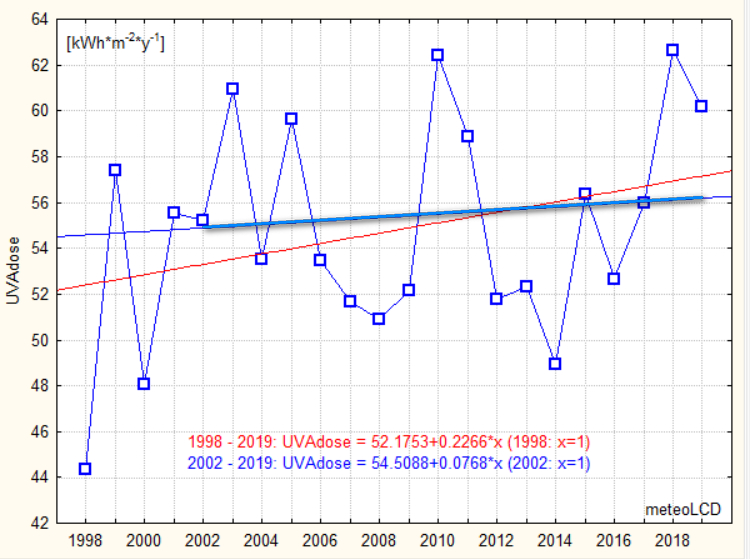
UVA dose of the year 2019: 60.2 KWh/m2
(some intermittent problems with internal temperature stabilization of the sensor; the influence seems minimal, so all readings have been kept)
mean +/- stdev:
1999 to 2019: 55.28 +/- 4.29 kWh*m-2*y-1
2002 to 2019: 55.55 +/- 4.26
2010 to 2019: 56.22 +/- 4.74 (last decade)
Trend from 2002 - 2018 is nearly flat.
The 2 independent measures of UVB and UVA doses all
point to a very slight increase since 2002, conforming to the increase of
total solar irradiance
(trend is +0.88 Kwh*m-2*y-1)
(End of measurements useable for trends in 2013. Measurements stopped in 2017).
Attention: only
78% of possible measurements available due to sensor downtime!
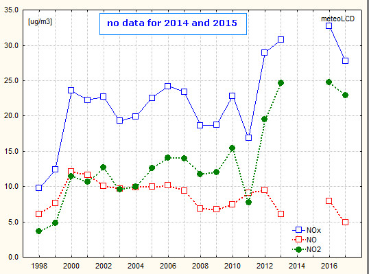
Comparison between yearly averages at Diekirch, Luxembourg-Liberté and
Vianden (rural)
[39]; Luxembourg and Vianden values derived by
inspection from graphs):
|
ug/m3 |
NOx | NO2 | NO | maximum of daily avg. NO2 |
| Diekirch | 28 | 23 | 5 | 62 |
| Luxembourg-Liberté | ~ 50 | ~ 82 | ||
| Vianden | ~ 10 | ~40 |
The NOx/NO measurements by the AC31M instruments from Environnement SA have
been stopped the 30 December 2017. The AC31M has reached its end of life.
see [11] which gives ~30% reduction from 1990 to 2005 for the EU-15 countries.


